

Before I get started here, I just wanted to give you, beloved reader of No Ceilings, an introduction to what I have vainly attempted to do in the article that you are hopefully about to read below. I, a novice programmer who has only ever successfully coded in HTML and R (having previously failed to learn Python) and hasn’t taken a statistics class in more than a decade, decided to create an analytical model for scouting. The article below is a mixture of a chronicle of what happened and a description of the result.
I hope the model turns out to be useful. At the very least, the worst-case scenario of describing my miserable failure might be entertaining to read.
I wrote the previous five sentences on December 2nd, 2025, for reference when this article comes out. They’re edited from the original (thanks, Jacob) but mostly represent my innocence at the start of this idiocy.
Although some self-editing was done out of order along the way (it’s in my nature), the sections of this article were primarily written chronologically. This shows the evolution of how I thought about proceeding with this project at key points along the way—or my rapid descent into madness, depending on your perspective.
Let’s see how it turns out.
*NOTE: All stats below are courtesy of RealGM, Synergy, or Sports Reference, unless otherwise noted. All stats are current as of 12/26/25.*
First of all, some acknowledgements. This piece would not have been possible without my brother, a brilliant computer scientist who helped me get this off the ground and immediately (and repeatedly) stopped me from driving the metaphorical car of this project directly into a brick wall.
It also wouldn’t have been possible without the No Ceilings team as a whole, of course—but especially my Deep Dives co-host for the No Ceilings NBA Draft Podcast, Paige Otto, who was the first person to discuss the five players who will be the focus of this exercise with me in depth. Ignacio Rissotto, our resident “actually good with data and Excel” guy, graciously took a ton of time out of his schedule to help me figure out where and how to begin. I shouted him out earlier, but I have to thank our newest writer and editor, Jacob LeRea, again, for editing this mammoth article. I also have to thank Tyler Rucker, who put up with me rambling for an hour on the day this idea first crossed my mind—and, in the process, really helped me to frame the direction I wanted to go with this exercise. I suppose I can forgive him for the many hours I wasted on this project because he encouraged me to go forward with it.
Now, speaking of that framing…
My goal with this project is to develop an analytical model that accurately captures and projects a prospect’s future NBA success. I’m starting this exercise with a very intentional sample size of 35 players; I don’t remember as much as I would like from my stats classes, but I do remember that a sample size under 30 is generally considered not statistically significant.
Those 35 players are the 30 players in the first round of my latest Big Board for No Ceilings, along with five players I currently have as second round picks—all of whom Paige and I have talked about on Deep Dives. Those five are meant to be as representative of a sample as five players can be (say it with me: small sample size). They include one player in each of the four categories I’m using to frame the exercise, the same four that Nathan Grubel and I talked about on the 10-year retrospective podcasts we did a few months ago: guards, wings, forwards, and bigs/centers. They are as follows:
I’m picking those five because I feel like they cover a lot of different bases and also represent a good mix of the kinds of prospects I tend to fall in love with too much during my evaluations. A point guard who can really pass and play defense? Check. A wing with a funky offensive game and good to great defense? Check; actually, two of them. A really mobile and athletic forward who mostly projects to play as a roaming deterrent defensively while throwing down gravity-defying dunks on the other end? Check. A center who blocks shots like crazy, makes great interior passes, and even has a bit of a jumper? Check.
It really doesn’t help that two of them (Stojakovic and Byrd) are from the Sacramento area (Carmichael and Stockton, respectively), which swings me in their favor even if only subconsciously—and in the case of Peja Stojakovic’s actual son, definitely more than subconsciously. If there are any players about whose games I could use a cold-water dousing to prevent ranking them too high, these five would be close to the top of the list.
Now, for why I’m writing this in the first place. When I first started writing about basketball professionally 10 years ago (dear God, I’m old now), I was almost entirely reliant on the cutting-edge analytics stats of that era. I’ve gotten more comfortable with evaluating film over time, to the point where I’ve fallen pretty far out of step with analytics. That feels off to me. I’m writing about sports in the first place because of Moneyball and Bill James, after all.
This is the part where you can blame Tyler Rucker. During our conversation, he mentioned that, drawing on his scouting and coaching background, he felt he needed to learn more about analytics to become more well-rounded. I entered the basketball space in precisely the opposite way, closer in time to taking those stats classes I mentioned earlier, and felt like I had to learn various plays and defensive schemes to make sense of all the film. Now, I’m going back to analytics to help bolster my film-watching and answer some of the questions I feel are most confusing to me, with defensive analysis at the top of the list.
Defense is still tricky for me to judge when evaluating a prospect; my biggest struggle is trying to determine how many of a player’s mistakes aren’t due to them screwing up, but rather are due to them continuing to play their part in a team-wide defensive scheme that fell apart somewhere else in the chain. I feel like I’ve gotten to the point where I’m pretty good at evaluating prospects on the offensive end. However, I think the second-most important principle in scouting (right behind the most important one, always having hope) is the ability to admit when you are wrong. It’s admittedly subjective, but anecdotally, the majority of the swings and misses in my scouting career have been in terms of defensive evaluation.
This is also anecdotal, but I feel like a decent chunk—if not most—of the basketball stats community agrees that the most commonly used advanced metrics are MUCH more accurate for offensive production than for defensive production.
Additionally, in terms of creating a valuable scouting model, I only know what I’ve learned from a few weeks of bothering my computer-science brother, my two stats classes in college, YouTube coding tutorials, my scouting background, and my knowledge of the more mainstream analytics-related statistics and models of this era. With all of that in mind, I’m expecting this model to be woefully inadequate in terms of defensive value. It would be great to have a solid answer to some of those questions, but I have to be realistic and acknowledge that defense will likely be the biggest hole in the early versions. Hopefully, though, the model will be good enough with the offensive stuff to make up for it and end up being useful at worst and really helpful (even elite) at best.
In other words, my goal here is to make my statistical model as similar to Isaiah Thomas as possible. Given that he’s my favorite player of all time, I suppose that this makes complete sense.
The first step for me in putting this together was getting all of the relevant numbers. Ignacio and my brother were both essential to this part of the process—Ignacio in showing me what I could do and patiently walking me through it, and my brother in doing the same for what I couldn’t do.
Once I’d passed that initial hurdle of how to gather the data, I decided to separate what I would do for the five second round prospects noted above, and the 30 remaining players in my sample (the Top 30 of my most recent Big Board). For the five, I decided to watch every possession on Synergy for each player this season, both on defense and on offense, to get as good a handle on their on-ball film as possible, as well as one complete game to evaluate their off-ball play on both ends. The sample size in the early season is too small to draw definitive conclusions—especially without many, or any, games in conference play—but I wanted to be as sure as possible about the film for those five before I figured out how to factor that into the model.
This is part of why I was so sure earlier that the defensive weighting would be the weakest part of this metric. On top of the fact that getting defense into a metric is widely recognized as more difficult, I was going to have to rely on my evaluation of a player’s defensive capabilities in some way while putting this together.
My own biases would factor into the selection and weighting of the stats, no matter how hard I tried to correct for them. If there is one thing that I learned from the many more psychology and neuroscience classes that I took in college than stats classes (or my precisely zero computer science classes), it’s that we’re all human all of the time. We all screw up constantly whenever we’re trying to do anything—whether we want to or not. The only thing I could do was my best, both in choosing inputs and in evaluating how prospects looked on film when defending in isolation or off-ball in a switching scheme.
Let’s get into those details now before the numbers start to come into play. At this point in the process, I have five factors going into the metric, which I’ll break down numerically in more detail in the next section. Those five factors are as follows:
-
Basic box score numbers. The building blocks of any metric.
-
Dean Oliver’s Four Factors: Effective Field Goal Percentage, Turnover Percentage, Offensive Rebounding Percentage, and Free-Throw Rate. Hard to go wrong with the classics.
-
Catch-all stat metrics, as available: your Win Shares, BPMs, WARs, VORPs, PERs, and so on; the ones that are public, at least.
-
Synergy numbers, weighted by position. Many of these numbers will have positional weights, but the weighing will be most prevalent with the Synergy numbers. To give an example, I’m more concerned about a point guard without a good pull-up mid-range jumper than I am about a defense-first center with the same weakness, and I want to make sure that those adjustments matter in the final number. On the other hand, I’m less worried about a point guard being good on the offensive glass than I am about a center. Having a strong off-the-dribble shooting game as a center is certainly a plus, don’t get me wrong; it’s just less important for determining that player’s NBA potential in my mind than it would be for a primary ball-handler.
-
Miscellaneous/Other. This generally encompasses anything else included in the metric. At this point in the process, these numbers comprise the takeaways from my film evaluation as described earlier, player age, and a vague “potential” stat that combines player age with my best guess of their potential to develop quickly. While plenty of players buck the trend and develop later, and while I firmly believe that prospect age is dramatically overvalued as an indicator, it is still relevant. It’s true more often than not that a 19-year-old will improve more over the next four years than a 23-year-old—if for no other reason than that the 19-year-old is no longer a teenager and therefore almost by definition will put on more weight and muscle over those years. The weights for some box score stats and Synergy numbers, along with the film evaluation and potential numbers, are the only subjective inputs I’m considering for the metric.
I have to give one last warning before we get to the meat and potatoes of this article. Put simply, there is a reason that I put “Model 0.0” in the title of the piece. This is not a final product. This is not even an inkling of the (idealized) final product. All of the inputs to the model are subject to change. This is primarily a journal entry detailing how I arrived at the fundamental, early-access version of what I hope the final numbers will be in the future.
In this moment, I can’t help but think of Bill James, one of the founding fathers of sabermetrics, whom I referenced earlier. Bill James has written many books and articles throughout his illustrious career. Still, it’s one of his terms from his glorious tome, The New Bill James Historical Baseball Abstract, that I hate the most that has stuck with me almost as much as anything else. I’m pretty sure it came from that book, although I couldn’t find it quickly on a glance-through; it’s very possible that it came from another book of his. If not, and I just hallucinated that memory, I refuse to take credit for the hideous term that you’re about to see.
“Imagenumbers.”
I hated the name when I first read it, and I still do, but it stuck with me like the theme song of a terrible commercial. It still feels weird to write about or talk about, but it conveys the concept so succinctly that I felt like bringing it up despite my revulsion.
I want these numbers to paint a picture that is hopefully worth a thousand words (more than that, given how long this article is already).
I want these numbers to tell a story.
Well, 35 stories, to be precise.
I’ll skip the part where I gathered a ton of data on the initial five and the full 35, put the numbers in a format I could understand, tried my best to digest the data, and came up with the catch-all numbers that I’m tentatively calling “Unweighted Prospect Score” (UPS) and “Weighted Prospect Score” (WPS) below. To everyone who made it this far: Thank you for reading; also, you’re welcome for saving you from what was by far the most tedious part of the process. For those of you who want to know more, I might share more details if there ends up being a v0.1 of this project; incredibly long story short, it came down to a lot of time in Excel and RStudio.
If I’ve done this correctly, the tables below should be downloadable and cover the input data outside the Synergy numbers and my miscellaneous/other factors noted above—I’ve got to keep a little bit of the secret formula to myself, at least for now. All of the inputs for the Unweighted Prospect Score are publicly available via RealGM.
Let’s start with the initial five. A key factor in my going with those five, beyond all the film I watched and how much I like them as prospects, is that they have all played more than 30 games of Division I college basketball. Even though the sample size of the film I watched specifically for this exercise was almost exclusively from this year, I watched all of them play last year and have at least some data in a sample size larger than 30 games when I include their previous seasons.
Simply put, this data won’t be as robust for the 18 freshmen in my Top 30—and therefore, as always, those players are going to be more heavily impacted by early injuries and fast or slow starts. That won’t be the case for our initial five.
This also, admittedly, dampens the impact of development on these numbers; averages from their first years of college hoops, when they were different players, will be included just as much as those from this season. That’s one of the many things that the Weighted Prospect Score attempts to solve in comparison to the Unweighted Prospect Score, but we’ll get into that later.
Now, after a ton of words and as many caveats as I can think of (my bad)…on to the numbers:
Those numbers are the numbers for the first three factors I mentioned above, plus the Weighted Prospect Score (we’ll get into much more detail on that number in particular in just a bit). The Unweighted Prospect Score, on the other hand, is the most straightforward math there is: I put all of the input numbers after that column, added them all up, and saw which total was the largest.
That number will serve as the control, not in the sense that I think it will translate fantastically or poorly to NBA success, but because I’ve done absolutely nothing to doctor those numbers with my own priorities when evaluating prospects. If the Unweighted Prospect Score control number turns out to be correlated with NBA success in a statistically significant way when I run the regressions later, great! It should be, seeing as it’s just all of the basic box score stats added together, plus Dean Oliver’s Four Factors, plus some of the most thoroughly reviewed and put-together advanced stats out there in the public sphere. If it does better than the version with my weights, though, I’d either need better weights or better eyes.
I want to go into the weights in some detail before I go any further.
I weighted all the factors to normalize them to a percentage baseline, from 0.00 (0%) to 1.00 (100%). With these weights, the prospect who is the best in the draft class in a specific area should have a score of close to or exactly 1.00 in that area, and a prospect who has taken zero off-the-dribble jumpers should have a score of 0.00 in that area.
In other words, I wanted both points per game and True Shooting Percentage to factor in, but not in a way that equates to the raw magnitude of the numbers. Antawn Jamison scored 18.5 points per game in the NBA, and Dennis Rodman scored 7.3 points per game; I don’t think anyone would agree that Antawn Jamison was automatically 2.5 times more valuable as a player than Dennis Rodman based on their scoring numbers.
Speaking of Dennis Rodman, his 16.4 rebounds per game over 506 games during the nine seasons he played in and around his 30s, including leading the league in six of those seasons, is much more of an outlier than any league-leading dominance from any scorer over the last 40 years. The weights attempt to reflect that.
Some of these weights will also be inversely proportional to the statistic in question. Those are pretty straightforward, too; for example, a lower Defensive Rating is better than a higher one. The control accounts for Defensive Rating by just adding the number as-is, but that’s not how I want it to go in the weighted version. That’s in addition to weighting to make sure that the two stats that are regularly near 100 (Offensive Rating and Defensive Rating) don’t drown out the rest of the statistical profile.
For those of you who might be worried about me putting my thumb on the scale too much: there are only three statistics out of 59 columns of data in the Weighted Prospect Score calculations that are purely my subjective opinion, titled as follows: Offensive Film Evaluation Ranking, Defensive Film Evaluation Ranking, and Potential Evaluation Ranking—all of which are ranked from 1-35. The Potential Evaluation Ranking is literally just their ranking on my most recent Big Board (which, for reference, I filled out in November) for the 35 players. Therefore, it’s identical to their position on my board from 1-30, and not so different for the initial five in the second round. Even if you think that that information shouldn’t be included because I have no right to call myself a scout, first of all, rude; second of all, the numbers that are entirely my own opinions are a small fraction of the many inputs to the Weighted Prospect Score.
For the deeper stats nerds, this is my fumbling effort to create weights that let me put the statistics that matter most to me in my own evaluations on a relatively similar scale before I add them to how they’re reflected in the Weighted Prospect Score. My idea there (and I’m pretty rusty on this and not great at it to begin with, so any corrections I receive from smarter people will be deeply appreciated and will absolutely be reflected in potential future versions) is that I can add them all together relatively easily without any one statistic influencing the data too much, and then regress the combined result against as many measures of NBA success as I can manage before I drag this process out to the point where I drive myself insane.
The basic idea is that the #1 overall pick should, in theory, have the highest Weighted Prospect Score; that player should project to be an NBA All-Star about 60% of the time, based on history. In the future, I would like to have a more directly z-score-based approach, where, in theory, a Weighted Prospect Score for a player who averaged 1.0 across the board would be somewhere around the #10 pick, a player who averaged 2.0 across the board would be one standard deviation better, and a player who averaged 0.0 across the board would be one standard deviation worse. In that model, the range of draftable prospects will almost certainly be tightly banded around 1.0; it might make more sense to make the projected #60 pick the 1.0 average across-the-board player, depending on how the data looks in a larger sample size, but that’s for another time.
(Everyone else: you can come back now.)
After doing this with the initial five, I did it with all of the first round picks. Ironically enough, I have now watched FAR more film of the five second round picks in the initial sample than I have of the Top 30 on my Big Board. At this point, I’m much more confident in the most subjective parts (my film and potential evaluations) for those five than I am for my assessment of my personal #1 overall pick going into this exercise, Darryn Peterson.
The one obvious note I have to make is that one of the players in my Top 30 (Karim Lopez) is not playing NCAA basketball this season. I’m hoping to break down the relative difficulty of playing against NBL competition versus high-level NCAA competition at some point. Since he is a single example for this exercise, though, I’m leaving parsing that difference to a future version of the model and just going with Lopez’s stats as if he were playing home games in Westwood this season instead of in New Zealand. I also gave him a placeholder BPM value of the exact median of the BPM totals for the college players, since BPM data is not available for the NBL (we’ll get into that column in more detail when we get to the regressions). Now that I’ve said that, here’s the expanded 35-player table:
Now, for the most nerve-wracking and vital part of the process: the regressions. Simply put, I have to figure out whether my Weighted Prospect Score metric does a better job of predicting NBA success than the Unweighted version, AKA the control variable. To try to figure that out, I had to build a list of NBA comparables for the players being scouted. I could then determine the college numbers for those prospects and their respective Weighted and Unweighted Prospect Scores.
For this version, I excluded the three subjective stats noted above entirely; I haven’t watched enough film of all of the NBA comparison players while they were (or were not) in college to assess their film accurately. The potential metric is entirely pointless because the goal here is to compare actual NBA production to how my model would have rated them entering the draft.
I went with six NBA comparables for each of the initial five, for a total of 30 NBA players. This would give me a statistically viable sample size and allow me to incorporate the NBA comps from my No Ceilings colleagues for our Preseason Draft Guide, where applicable. In total, 20 of the comps are my own, with 10 from the No Ceilings crew—nine from the Preseason Draft Guide, and an Andrej Stojakovic/Jaime Jaquez Jr. comp from Corey Tulaba that made me disgusted with myself for not having thought of it earlier.
I could have come up with film scores for Jaquez Jr. and a few of the other NBA comps, but I was already worried enough about those subjective measures being in the Weighted Prospect Score. I wasn’t going to try to do the same for players who had already had some degree of success (or failure) in the NBA.
Admittedly, I had also poured way too much time into just the set-up work at this point in the process to even dream of coming up with six comps for every single one of the Top 30 players on my board. Unfortunately, the number of comparisons needed for me to feel truly satisfied with the experimental results was just too large to put together for v0.0 of this model, unless I wanted to keep working on it until 2043.
Here is the table containing the Weighted Prospect Scores and Unweighted Prospect Scores from the NCAA playing data of the 30 NBA comparables for our initial five. As a quick note, one of the NBA comparables (Ariel Hukporti) did not play NCAA basketball; I treated his stats the same as Karim Lopez’s from the previous table. Also, two of the comps (Kyle Lowry and Jameer Nelson Sr.; wow, my back started hurting as soon as I wrote that “Sr.” at the end) played their college ball long enough ago that I couldn’t find complete advanced stats for them; the Offensive and Defensive Ratings for Nelson are from his final two college seasons, and I used 0.5 as a placeholder (to represent the 50th Percentile; unscientific, I know, but it was the best thing I could think of to do when I was this deep down the rabbit hole) for their missing Synergy numbers so that those numbers wouldn’t be skewed by a 0.0 in that column. Now, onto the NBA comparison players:
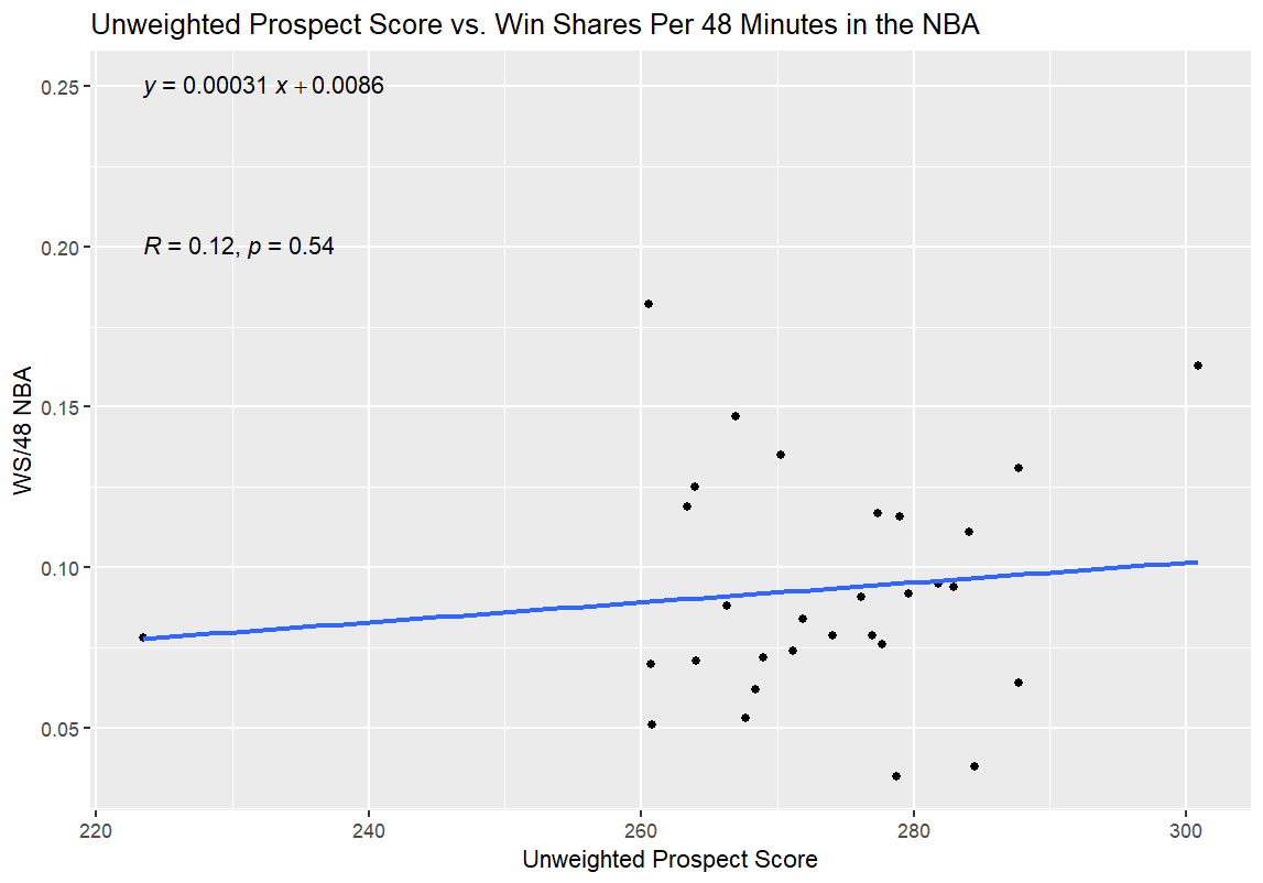
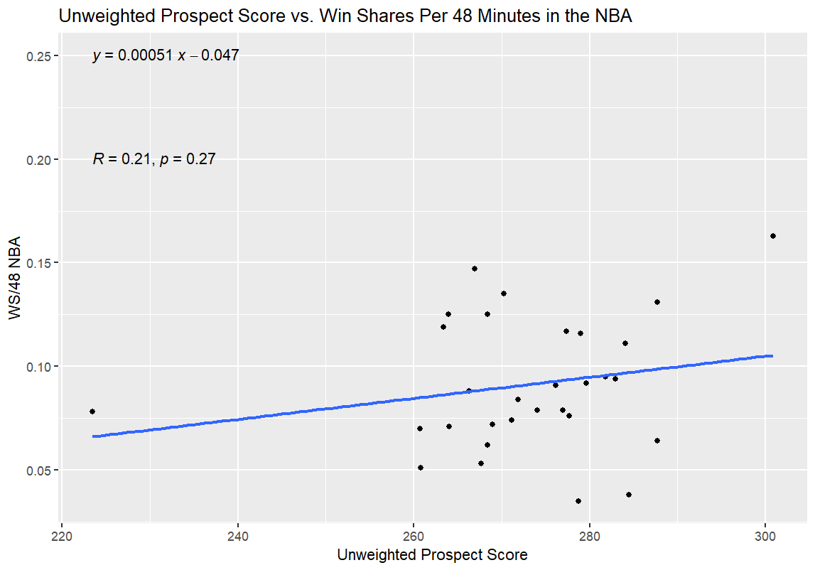
And finally, time for the regressions. For the first one, I regressed Unweighted Prospect Score and Weighted Prospect Score against Win Shares per 48 Minutes (WS/48) as a standard for NBA production; in theory, this would allow me to see how good the two college stats metrics I had slapped together were at projecting a player’s NBA efficacy. My hypothesis going in was that both college numbers would have a predictive effect on the NBA production of those players, as measured by WS/48, but that the Weighted Prospect Score would be more closely correlated with WS/48 than the Unweighted Prospect Score. If it turns out that way, I’ve at least got something to build on going forward. If Unweighted is predictive and Weighted isn’t at all, or if Unweighted is equally or more predictive, then I have to go back to the drawing board.
If neither measure is correlated with NBA success at all, then I have to check my code, because, logically speaking, that seems so unlikely as to be rarer than lightning striking the same place five times. It would essentially indicate that none of the basic box score stats, Four Factors, or publicly available advanced stats for college players have any predictive value at all in terms of a player’s NBA success. I can’t dismiss the possibility entirely, in theory; however, my fourth-grade English teacher (one of the best teachers I’ve ever had; shout-out to you, Mrs. Burton) taught me to be skeptical, and it defies belief that every basic box score number from college play means nothing in terms of NBA translation—especially since that had already been proven not to be the case as of more than a decade ago when I first started reading about basketball analytics.
Alright, moment of truth time; here are the results from the first round of regressions:
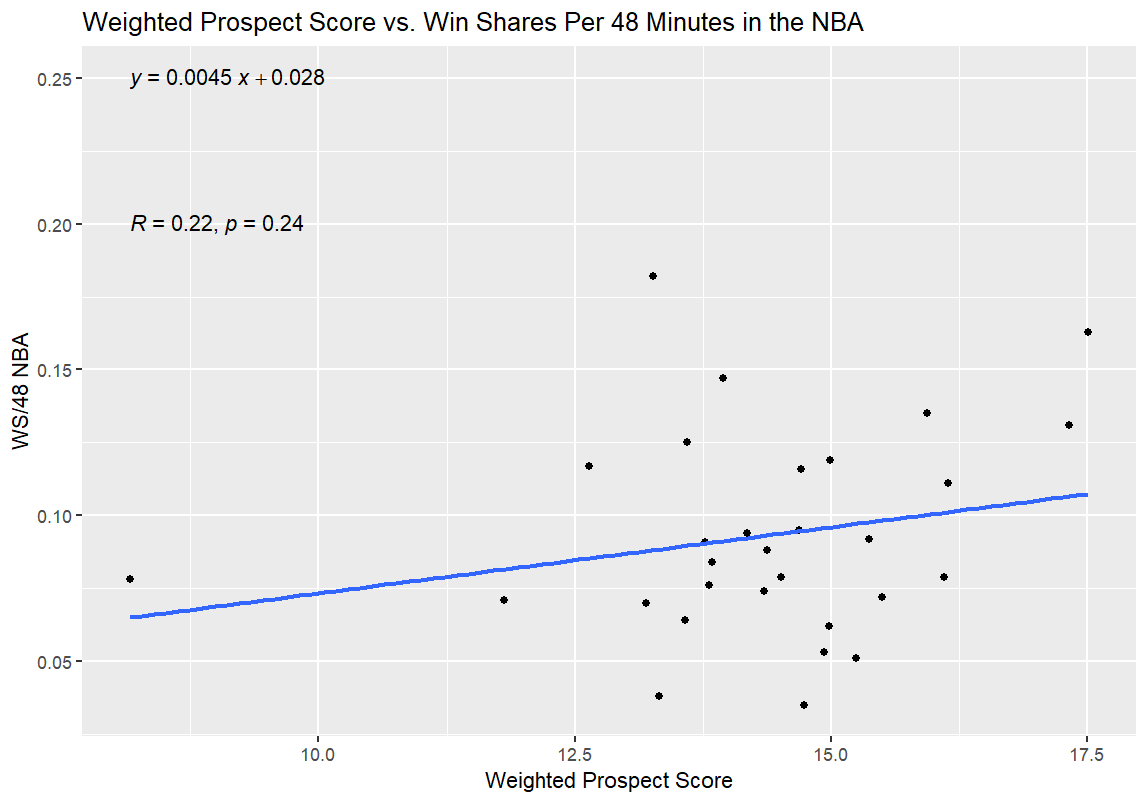
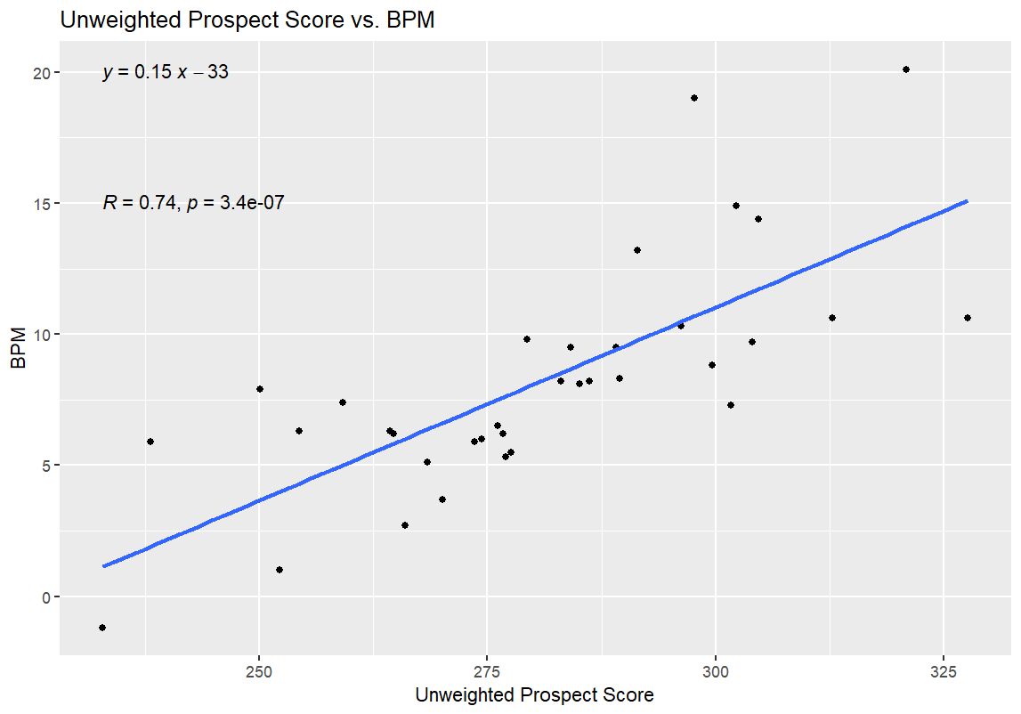
I’ll get into what (I think) all of this means in the next section, but I have one more set of graphs for all of you before that. After the first round of regressions, I also ran a second round with the 35 prospects for the 2026 NBA Draft. I used BPM for this regression, since obviously the NBA WS/48 data wasn’t available. I didn’t use WS/40 for this data, as WS/40 is one of the inputs for the Weighted Prospect Score; I didn’t want to muddy the data any more than I already had by regressing the Weighted Prospect Score against one of its inputs. Here are those results:
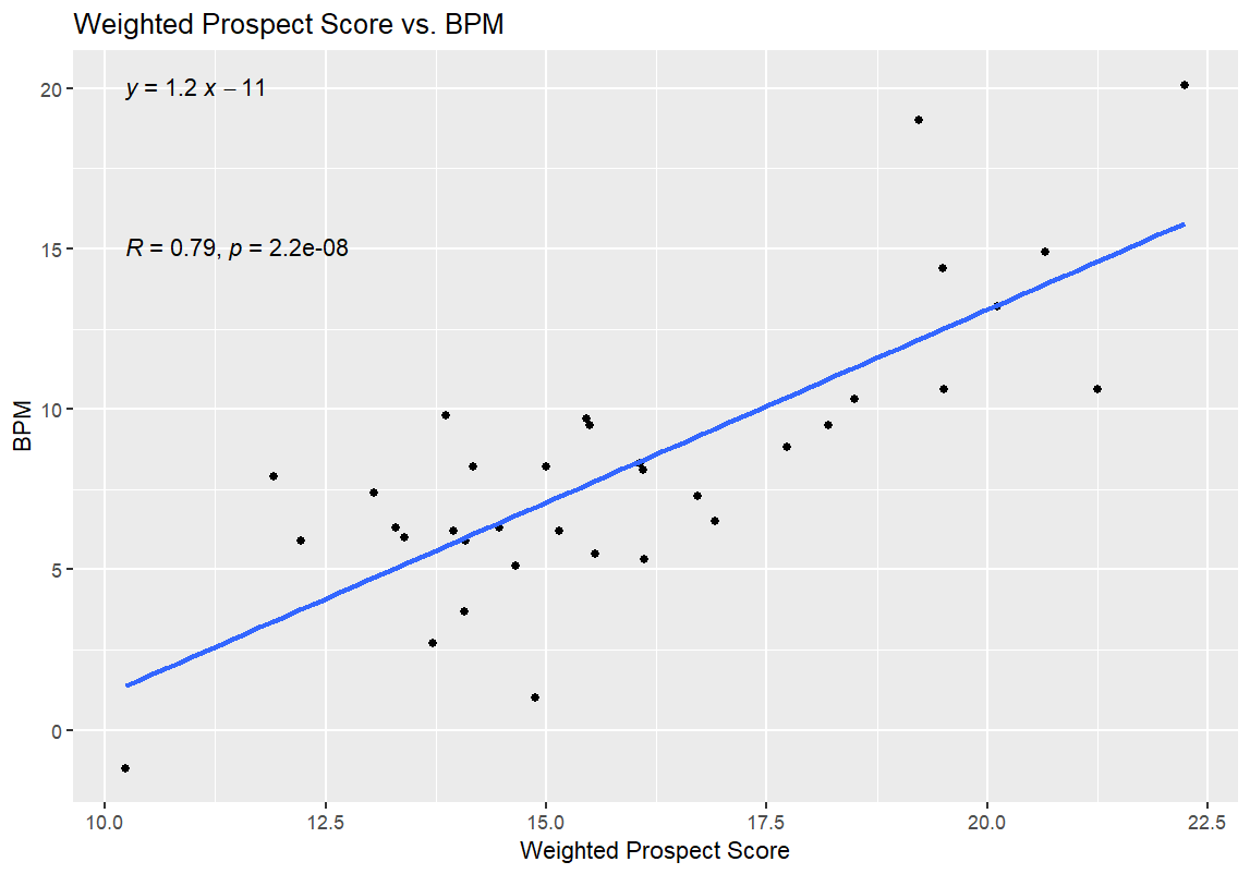
Let’s start with the good news: the Weighted Prospect Score formula works!
I think.
Here’s the breakdown for those of you who aren’t as versed in statistics (for those of you who are, you’re probably already screaming about me attempting to draw any conclusions whatsoever from the first two graphs).
The linear algebra formulas in each of the four graphs above indicate the relationship between the numbers on the x and y axes. In other words, it gives the formula for the blue line, which approximates how much the stat on the y-axis increases with respect to the x-axis.
The R and p numbers are the meat of the linear regressions. Essentially, the R value measures the strength of the correlation between two variables, ranging from -1 to 1, with -1 indicating a perfect inverse correlation (e.g., y = -x) and 1 indicating a perfect positive correlation (e.g., y = x). The p-value is to predict how likely it is that the relationship is purely coincidental—the root of the phrase “correlation does not equal causation,” in other words. A p-value of less than 0.05 is considered significant (meaning that there is a 95% chance or greater that the correlation is not a coincidence).
The best news, from my perspective, is that the Weighted Prospect Score outperformed the control variable, the Unweighted Prospect Score, on both tests; the WPS had a higher R value and a lower p value. Furthermore, the UPS was correlated with better performance in both tests—meaning that Mrs. Burton’s advice was just as right as I always knew it was, because the seemingly impossible outcome of no correlation at all didn’t come to pass.
Now, here’s the bad news: the p-values for the NBA comparisons aren’t statistically significant. To me, this means something unfortunate but not model-breaking as a first step. While the p-values tell me that my data is garbage, in so many words, I think that my biggest issue at the moment is my limited sample size. It’s possible that the correlation between NBA success as measured by WS/48 and WPS did mean a correlation—I just couldn’t feel confident enough that said correlation was lucky or not without a lower p-value. That’s especially true since most statisticians use R² instead of R, and my R² for the Weighted Prospect Score is only R² = 0.048, which is a pretty weak correlation between the two numbers.
To be clear: it’s a massive win that the WPS/BPM graph has such a low p-value, and an even bigger win that it has a lower p-value than the UPS/BPM graph, and a win that the R and R² values on those regressions are pretty strong, and that WPS once again beat out UPS. It means that the WPS value shows statistical significance for success at the college level, beyond what’s explained by the UPS number. In theory, it shouldn’t be all that surprising that both numbers should have been correlated with BPM—ultimately, all of the advanced metrics of this or any era are predicated on a player’s performance on the court, and being good at basketball leads to better numbers on traditional box score stats and advanced stats alike. WPS doing better than UPS on that measure might be due to something as simple as WPS considering lower Defensive Ratings and TOV% numbers as positives rather than negatives, like UPS does, but figuring that out would require more digging.
With the p-values being what they are for the NBA comparison regressions, though, I can’t draw any solid conclusions about whether or not my WPS stat has any predictive value for a player’s NBA success.
Then again, that is kind of why I wanted to get started on this project in the first place: I wanted to create a model that could incorporate my scouting philosophy and film watching into a metric that would predict NBA success. Scouts have been trying to do that with and without models since the first NBA Draft in 1947. There was no way that my model was going to be good enough on the first try; the ideal would be to get something passable after many, many, many iterations, and then keep refining it from there.
Still, all in all, I’m pretty happy with where I am after taking the first step on that journey.
That last sentence was where I was at with the piece when I let poor Jacob know that the last two sections of the article were finally ready for editing.
Then, I tried to go to sleep, and couldn’t (those who know me well know that this is not exactly a rare occurrence).
I thought about it some more and decided that the p-value thing for the NBA comparisons didn’t sit right with me.
I tweaked the weights on the WPS deep into the early morning hours. I was close to figuring it out. I was really close:
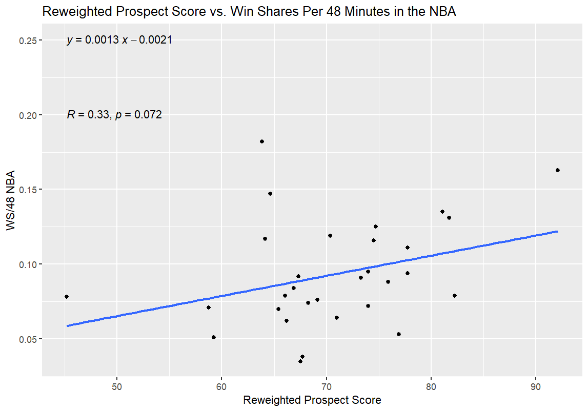
No matter how many tweaks I made to the weights from here, though (and trust me, I spent way too much time on this part of the project for the sake of my own sanity), I couldn’t get much closer to a statistically significant correlation than this.
Then, I realized the truth.
I had a Luke Kornet problem.
I thought Luke Kornet made quite a bit of sense as an NBA comparable for Nate Bittle, but there was a specific problem that Luke Kornet presented that nobody else in the sample size had.
See, Luke Kornet is the dot at the top of the y-axis. He had a middling Prospect Score by the Weighted and Reweighted versions of the stat, and his middling numbers (relative to the rest of the sample size) are certainly a part of why he went undrafted out of Vanderbilt. However, he has been fantastically effective at the NBA level—especially over the last five seasons, which have been his best seasons by WS/48 and have seen him play by far the most minutes as well, indicating that he wasn’t just a small sample size wonder in recent years.
I was torn about whether to remove Kornet from the sample, even though it clearly solved my p-value issue. On the one hand, the best possible outcome for this model would be an ability to find undervalued prospects like Luke Kornet.
On the other hand, his massive outlier status could mean something entirely different. Luke Kornet shot a high volume of three-pointers in college (with a .511 3PAr), and hit them at a 32.0% clip. He shot a high volume of three-pointers over his first four NBA seasons (with a .631 3PAr) and hit them at a 32.8% clip. In the five seasons since then, he has cut out three-pointers almost entirely (.028 3PAr)—and his efficacy has increased dramatically. In terms of both his shot diet and his effectiveness, the Luke Kornet who entered the NBA is an entirely different player than the player he has been since he stopped tossing up triples.
With that in mind, I decided to cheat and use the WS/48 numbers for Kornet’s first four seasons, excluding his dramatic mid-career change in profile. It was definitely cheap, but to be entirely honest, the Kornet of his first four seasons is a better comp for Nate Bittle anyway. Now, I could see if muting my outlier made my p-value a bit more palatable:
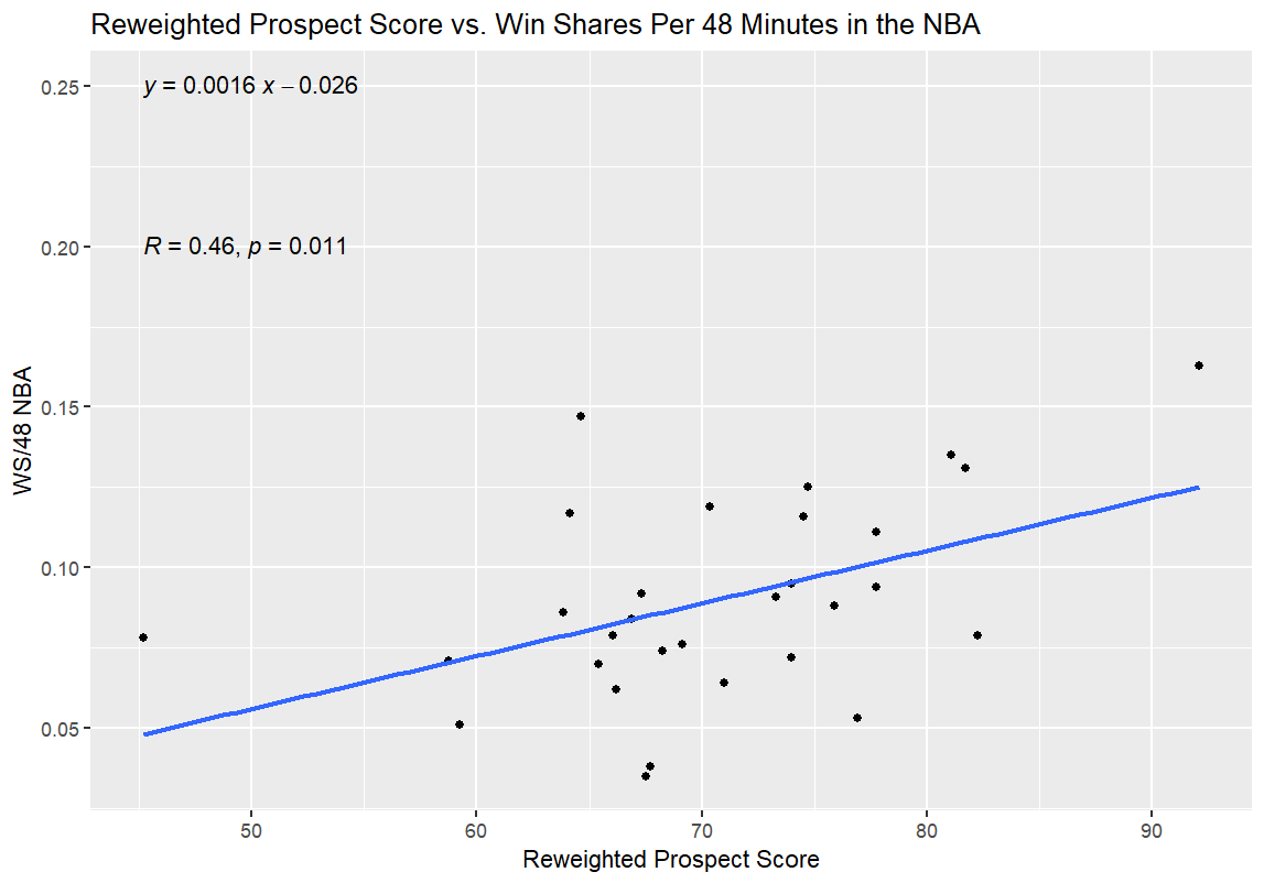
And…there it was. After kneecapping my biggest outlier by ignoring his (presumably) coaching-influenced complete change in shot diet, I found a p-value indicating that the new, Reweighted Prospect Score (RWPS) was correlated with NBA success in a statistically significant way, with a much stronger correlation between the new stat and NBA performance, as measured by R and R². I could go to bed, in theory.
For reference, removing Kornet and Frank Mason III (the opposite of Kornet as the most significant outlier negatively speaking in terms of the difference between his college and NBA production) from the sample entirely had a similar effect to the graph above. However, it reduced my sample size to below 30.
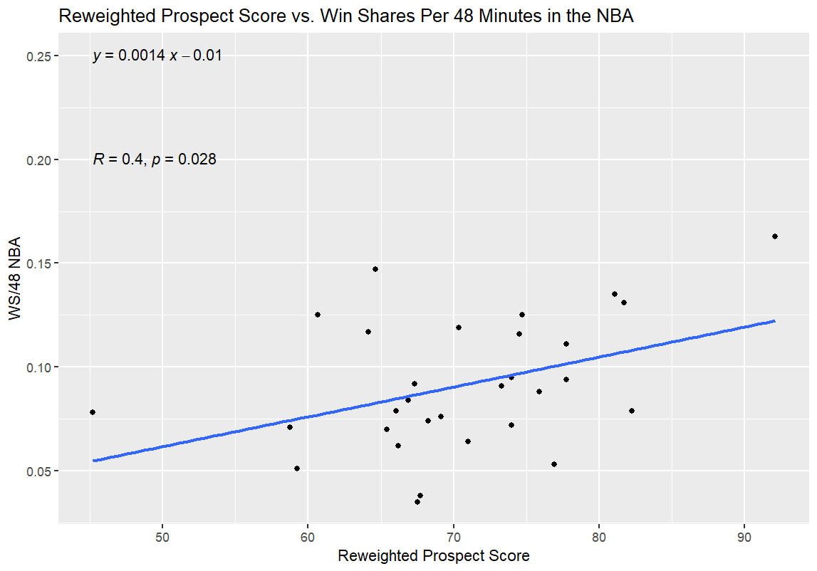
I re-ran everything at a more reasonable hour, with Sandro Mamukelashvili as the sixth Bittle comp instead of Kornet; as it turns out, he was a strong outlier as well, but nowhere near as much of one as Kornet in terms of breaking the data:
Now that I’d redone the WPS entirely, I also re-ran the WPS/BPM comparison from earlier, updating the WPS numbers for the college prospects in the 2026 NBA Draft with the weights used in the Reweighted Prospect Score:
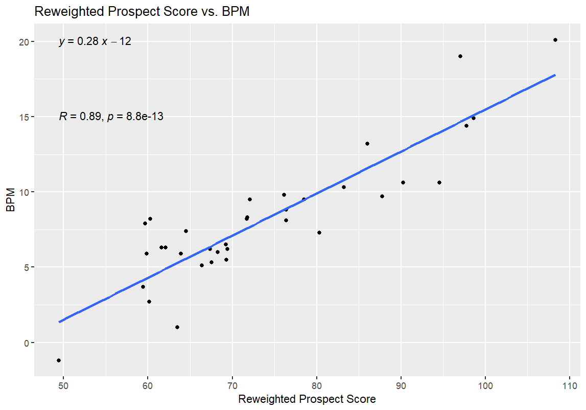
The higher R value and lower p-value here, as opposed to the original, further support the conclusion that the Reweighted Prospect Score is more valuable as a predictive tool than the original Weighted version. Just to check all of my boxes, here are the updated 35-player table for the 2026 NBA Draft prospects and the NBA comparison players with their new, Reweighted Prospect Scores:
As long as this article was, this is only the tip of the iceberg in terms of where I’m hoping to go with this project (assuming that our readership and/or the other editors on the No Ceilings team will put up with it). My brother and Ignacio have both made the gigantic mistake of agreeing to keep talking to me about this; we’ll see how many of my ideas around this metric come to fruition.
The obvious next step for this project, in my mind, is to read as much academic literature as possible to brush up on and improve my statistics knowledge.
After that, several stats weren’t included in the initial Weighted/Unweighted Prospect Score calculations purely because I took way too much time setting up the first round of regressions to include and weight all of them. Those will be added to future versions. To be more specific, I want to add more possession-based rate stats (like various Per 100 Possessions and Per 40 Minutes stats) to account for good players playing limited minutes on loaded squads.
The next step would be to try to expand the comparisons of the Prospect Scores to potential NBA translations. My first assumption is that I would use some version of the Similarity Scores on Basketball Reference to find more NBA players with comparable college stats to the 35 players I discussed here, and see how well their Weighted Prospect Score translates to their NBA success.
On a more basic level, there are quite a few columns of data that I entered by hand rather than troubleshooting a more complicated code to move data from one place or program to another. The most boring parts of future updates for me will just be making sure as many of those things as possible are implemented in code, so I can expand to cover more prospects. I’ll try to make sure that all the coding is up to snuff as best as I can, with a bit of help from my friends.
After that, I would ideally expand the metric to reflect the competition the players in question faced more accurately; I would start with SRS off the top of my head and add other stats before I would be willing to call that part ready to go. After that, I would try to expand to all of college basketball and then other leagues. I could try to assign weights to each league to see which are most comparable to the NBA and/or NCAA ranks. This, of course, will be a lot easier to do with the Unweighted version since it doesn’t include any subjective numbers and, therefore, doesn’t require me to watch a lot of film on the prospects in question. However, since the goal of the project is to make the Weighted Prospect Score as helpful as possible, I’ll have to put in the legwork to get the result I’m hoping for from all of this.
For now, though, I think it’s time to call it a wrap on Model v0.0. We’ll see what, if anything, I can come up with on this in the future. I’m going to take a breather right now, but I’m happy that I decided to challenge myself and give this project a shot. At the very least, I learned a lot.
It’s always worth it to learn more and improve when you can.